Data Wrangling
In this chapter, we will see the following:
- DataFrames in Python with Pandas
- Datetimes and indexing
- Aggregating, transforming, and joining data
- Missing data and imputation
The dataset used in this Chapter comes from the Bureau of Transportation Statistics .
Introduction to Pandas
import pandas as pd
import numpy as np
import matplotlib.pyplot as plt
One might think that we have everything that we need to work with data. We can read data with built-in Python functions and we can store and manipulate that data with Numpy. Numpy is based around the Array, and Pandas is based around the DataFrame. Unlike the Array, the Dataframe treats each axis differently, with named columns and indexed rows. Pandas does this under the assumption that a DataFrame holds a large sample of a limited number of variables. Each column corresponds to a variable, while each row corresponds to an individual, time-point, or other index for repeated data.
Due to this presumption, Pandas is able to optimize operations such as indexing, aggregation, and time series statistics. It also has great Input/Output tools for reading delimited data, working with databases, and HDF5 data. Pandas is built around the data types: DataFrames, Series. Roughly, a Series is a list of indices and values (think of a time series where the datatime is the index), and a DataFrame is a dictionary where the keys are the column names and the values are entire Series, and these Series have a common index. This is a high-level overview of Pandas, and for more syntax details see the panda docs
Series
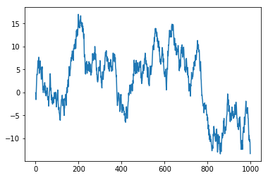
Let’s simulate a Brownian motion so that we can discuss Series objects. You can see a plot of this below, we will go over data visualization in the next chapter.
T = 1000
innov = np.random.normal(0,1,T)
brown = np.cumsum(innov)
plt.plot(brown)
plt.show()
Let’s suppose that the above simulation represents the change in a stock price starting from Jan 1, 2015. Pandas provides a tool for making sequences of datetimes; the following makes a DateTimeIndex object.
days = pd.date_range('1/1/2015',periods=T,freq='d')
We will return to datetime functionality in Pandas later. Another option
for working with datetimes is the datetime package, which has the
date, time, and datetime types and a timedelta object for increments of
time. To see the specifics of the datetime package you can look at
the datetime documentation
The resulting list contains the dates, for example,
days[600]
Timestamp('2016-08-23 00:00:00', freq='D')
We can initialize a series with a 1D array and an index sequence. If you omit the index then it will index with the row number. You can also initialize with dictionaries where the index values are the keys and the values are the data.
stock = pd.Series(brown,index=days)
The Series object should be thought of as a vector of data where each value is attached to an index value. Series operations will preserve the indices when they can. You can slice a series as if it were an array; in the following, we look at every seventh day in the first 100 days.
stock[:100:7]
2015-01-01   -0.132526
2015-01-08    3.900432
2015-01-15    7.371181
2015-01-22    6.224340
2015-01-29    3.449301
2015-02-05    1.346746
2015-02-12    2.084879
2015-02-19   -0.752967
2015-02-26   -0.983502
2015-03-05   -0.575965
2015-03-12    1.140087
2015-03-19   -2.205040
2015-03-26   -2.214539
2015-04-02   -1.170000
2015-04-09   -1.984565
Freq: 7D, dtype: float64
Due to the indexing, we can also think of this as a dictionary, as in the following.
stock['2016/7/27']
11.191250684953793
One of the key features that makes the series different from an array is that operations between two series will align the indices. For example, suppose that we have bought 100 shares of another stock on Jan 1, 2016, which we can simulate as well. As usual, since we are reusing code, let’s wrap it up in a function which we could put in a module.
def stock_sim(T,day1):
    """Simulate a stock for T days starting from day1"""
    innov = np.random.normal(0,1,T)
    brown = np.cumsum(innov)
    days = pd.date_range(day1,periods=T,freq='d')
    return pd.Series(brown,index=days)
T = 1000 - 365
day1 = '2016/1/1'
stock_2 = stock_sim(T,day1)
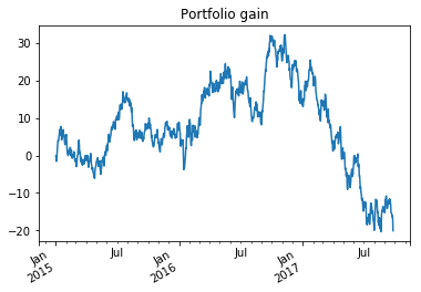
For each date we would like to see the difference between the value of the portfolio and the amount we spent on the portfolio. This is proportional to the sum of the two changes in stock price since we have bought even amounts of each stock.
portfolio = stock.add(stock_2,fill_value=0)
stock and stock_2 have different lengths but we are able to add
them because the indices can be matched. So after 2016 the change in
value of stock 2 is added to stock 1 since that will correspond to the
change in portfolio value. We had to specify a fill_value of 0
otherwise it would try report the portfolio value as missing before
2016. We can plot this.
# See next chapter
ax = portfolio.plot(title="Portfolio gain")
ax.figure.autofmt_xdate()
plt.show()
Dataframe
You should think of a dataframe as a collection of series objects with a common index. Each series in the dataframe has a different name, and they should be thought of as different variables. We can initialize the dataframe with a dictionary mapping names to series objects.
port_df = pd.DataFrame({'stock 1':stock,'stock 2':stock_2,'portfolio':portfolio})
If we had passed arrays instead of series then the default index of the
row numbers would be used. You can also pass a 2D array and specify the
indices and columns arguments. There are other ways to
initialize a dataframe, such as from lists of tuples and lists of
dictionaries.
We can view the first few rows of any dataframe with the head
method.
port_df.head()
| stock 1 | stock 2 | portfolio | |
|---|---|---|---|
| 2015-01-01 | -0.132526 | NaN | -0.132526 |
| 2015-01-02 | -0.087030 | NaN | -0.087030 |
| 2015-01-03 | -1.578688 | NaN | -1.578688 |
| 2015-01-04 | -0.240958 | NaN | -0.240958 |
| 2015-01-05 | 1.170581 | NaN | 1.170581 |
We see that stock 2 was filled with NaN values. We can also get at the indices and names via
print(port_df.index[:7])
print(port_df.columns)
DatetimeIndex(['2015-01-01', '2015-01-02', '2015-01-03', '2015-01-04',
               '2015-01-05', '2015-01-06', '2015-01-07'],
              dtype='datetime64[ns]', freq='D')
Index(['stock 1', 'stock 2', 'portfolio'], dtype='object')
Accessing elements in a dataframe differs from arrays in the following ways:
- dataframes act like dictionaries from the column names to the column
- slicing is done over the row indices
- to
port_df['stock 1'].head() # this returns the column
2015-01-01   -0.132526
2015-01-02   -0.087030
2015-01-03   -1.578688
2015-01-04   -0.240958
2015-01-05    1.170581
Freq: D, Name: stock 1, dtype: float64
port_df['2015/1/1':'2016/1/1'].head() #this returns a slice of rows
| stock 1 | stock 2 | portfolio | |
|---|---|---|---|
| 2015-01-01 | -0.132526 | NaN | -0.132526 |
| 2015-01-02 | -0.087030 | NaN | -0.087030 |
| 2015-01-03 | -1.578688 | NaN | -1.578688 |
| 2015-01-04 | -0.240958 | NaN | -0.240958 |
| 2015-01-05 | 1.170581 | NaN | 1.170581 |
Boolean fancy indexing works in the place of the slice above as well, for example, we can select rows with a boolean series,
port_df[port_df['portfolio'] > port_df['stock 1']].head()
| stock 1 | stock 2 | portfolio | |
|---|---|---|---|
| 2016-01-01 | 8.154289 | 0.702001 | 8.856290 |
| 2016-01-12 | 3.746795 | 0.412568 | 4.159364 |
| 2016-01-13 | 1.930705 | 0.585910 | 2.516615 |
| 2016-01-18 | -2.250490 | 0.158522 | -2.091968 |
| 2016-01-19 | -1.874360 | 0.796581 | -1.077779 |
which will find the elements in which the portfolio is better off than just our share in stock 1. The comparison between the portfolio and stock 1 is not quite fair because we invested more money in the portfolio. We can create new columns via the following assignment,
s1sim = port_df['stock 1'].add(port_df['stock 1']['2016/1/1':],fill_value=0)
port_df['stock 1 sim'] = s1sim
port_df[port_df['portfolio'] > port_df['stock 1 sim']].head()
| stock 1 | stock 2 | portfolio | stock 1 sim | |
|---|---|---|---|---|
| 2016-01-16 | -2.004913 | -1.310433 | -3.315347 | -4.009827 |
| 2016-01-17 | -2.863114 | -0.532889 | -3.396003 | -5.726228 |
| 2016-01-18 | -2.250490 | 0.158522 | -2.091968 | -4.500980 |
| 2016-01-19 | -1.874360 | 0.796581 | -1.077779 | -3.748719 |
| 2016-01-20 | -1.835044 | 1.822567 | -0.012477 | -3.670089 |
We added the value of stock 1 after 2016 to all of stock 1 to see what
the price would be if we invested in stock 1 again on Jan 1, 2016. If we
wanted to select instead a specific date, we would need to use the
loc method,
port_df.loc['2016/7/27']
stock 1        11.191251
stock 2         2.867483
portfolio      14.058734
stock 1 sim    22.382501
Name: 2016-07-27 00:00:00, dtype: float64
We can select and slice the dataframe as if it were a Numpy array using
the iloc method,
port_df.iloc[400:405,0:3]
| stock 1 | stock 2 | portfolio | |
|---|---|---|---|
| 2016-02-05 | -3.581697 | 6.968880 | 3.387182 |
| 2016-02-06 | -3.854760 | 6.472026 | 2.617266 |
| 2016-02-07 | -2.697462 | 7.555933 | 4.858471 |
| 2016-02-08 | -4.389190 | 10.106156 | 5.716965 |
| 2016-02-09 | -4.027021 | 8.067919 | 4.040898 |
Other things to be aware of are
- the
infomethod which provides the types and information of the columns, - many elementwise Numpy operations can be performed on series and
dataframes, such as
np.exp - Pandas has many of the same descriptive statistics such as
dataframe.mean()includingmin, max, std, count,...
We can see many of the descriptive statistics with the describe
method.
port_df.describe()
| stock 1 | stock 2 | portfolio | stock 1 sim | |
|---|---|---|---|---|
| count | 1000.000000 | 635.000000 | 1000.000000 | 1000.000000 |
| mean | 2.209039 | 8.755110 | 7.768534 | 2.802033 |
| std | 6.782089 | 9.029220 | 11.534137 | 12.119164 |
| min | -13.394813 | -14.372408 | -20.329462 | -26.789627 |
| 25% | -2.834049 | 3.965685 | 0.280122 | -4.962457 |
| 50% | 3.748605 | 11.666626 | 7.178422 | 4.646818 |
| 75% | 7.014775 | 15.381508 | 16.705302 | 10.896449 |
| max | 16.995441 | 23.052934 | 32.141200 | 29.696000 |
Wrangling data with indices
Reading data and datetime indexing
In this section, we will go over reading data with Pandas and datetime functionality. This is meant to explain why these tools exist and their basic functionality. For more detail, look at
import numpy as np
import pandas as pd
Pandas is especially useful because of its excellent Input/Output (I/O)
functions. The read_csv command has a few different ways of working.
If you specify that you want an iterator, with the iterator argument,
then you can get something that works like the CSV reader object. You
can also specify a chunksize, and then it returns an iterator that will
read the file in chunks (the first k likes, then the next k, etc.),
which is great for files that you cannot store in memory. By default
read_csv loads the file all at once. For example, we could read in all
of the following data file:
colnames = ['Origin','Dest','Origin City','Dest City',
        'Passengers','Seats','Flights','Distance','Date','Origin Pop','Dest Pop']
flights = pd.read_csv('../data/flight_red.tsv',sep='\t',header=None,names=colnames)
flights.info()
<class 'pandas.core.frame.DataFrame'>
RangeIndex: 1140706 entries, 0 to 1140705
Data columns (total 11 columns):
Origin         1140706 non-null object
Dest           1140706 non-null object
Origin City    1140706 non-null object
Dest City      1140706 non-null object
Passengers     1140706 non-null int64
Seats          1140706 non-null int64
Flights        1140706 non-null int64
Distance       1140706 non-null float64
Date           1140706 non-null int64
Origin Pop     1140706 non-null int64
Dest Pop       1140706 non-null int64
dtypes: float64(1), int64(6), object(4)
memory usage: 95.7+ MB
Let’s suppose that we did not want to work with over 1 million rows at once, and will instead just work in chunks. We can use the chunksize argument, which will then create an iterator that will yield DataFrames with that number of rows.
flights_it = pd.read_csv('../data/flight_red.tsv',sep='\t',header=None,
                         chunksize=100000, names=colnames)
flights = next(flights_it)
flights.shape
(100000, 11)
We have a dataframe with the same dtypes that we see from the output of
info() above, but with 100,000 rows. Let’s look at the head of this
dataframe.
flights.head()
| Origin | Dest | Origin City | Dest City | Passengers | Seats | Flights | Distance | Date | Origin Pop | Dest Pop | |
|---|---|---|---|---|---|---|---|---|---|---|---|
| 0 | MHK | AMW | Manhattan, KS | Ames, IA | 21 | 30 | 1 | 254.0 | 200810 | 122049 | 86219 |
| 1 | PDX | RDM | Portland, OR | Bend, OR | 5186 | 6845 | 185 | 116.0 | 200508 | 2084053 | 140962 |
| 2 | PDX | RDM | Portland, OR | Bend, OR | 2781 | 4650 | 155 | 116.0 | 200508 | 2084053 | 140962 |
| 3 | PDX | RDM | Portland, OR | Bend, OR | 66 | 70 | 1 | 116.0 | 200502 | 2084053 | 140962 |
| 4 | PDX | RDM | Portland, OR | Bend, OR | 3791 | 5143 | 139 | 116.0 | 200502 | 2084053 | 140962 |
There are several other similar methods for reading filetypes other than
CSV. For example, read_excel, read_hdf, read_stata, read_sas will
read excel, HDF5, Stata, and SAS files. We will return to reading JSON
and HTML files later, but will generally not use Pandas for these.
If we look at the Date column, we see that this is currently a string
(called an Object in Pandas—this is related to json). It should be a
date, so let’s convert it using pd.t_datetime.
flights['Date'] = pd.to_datetime(flights['Date'],format='%Y%m')
flights.head()
| Origin | Dest | Origin City | Dest City | Passengers | Seats | Flights | Distance | Date | Origin Pop | Dest Pop | |
|---|---|---|---|---|---|---|---|---|---|---|---|
| 0 | MHK | AMW | Manhattan, KS | Ames, IA | 21 | 30 | 1 | 254.0 | 2008-10-01 | 122049 | 86219 |
| 1 | PDX | RDM | Portland, OR | Bend, OR | 5186 | 6845 | 185 | 116.0 | 2005-08-01 | 2084053 | 140962 |
| 2 | PDX | RDM | Portland, OR | Bend, OR | 2781 | 4650 | 155 | 116.0 | 2005-08-01 | 2084053 | 140962 |
| 3 | PDX | RDM | Portland, OR | Bend, OR | 66 | 70 | 1 | 116.0 | 2005-02-01 | 2084053 | 140962 |
| 4 | PDX | RDM | Portland, OR | Bend, OR | 3791 | 5143 | 139 | 116.0 | 2005-02-01 | 2084053 | 140962 |
Converting this to datetime makes each individual entry a Timestamp object.
ts = flights.loc[0,'Date']
ts
Timestamp('2008-10-01 00:00:00')
The Timestamp should be thought of as a point in time, and it can have resolution down to the nanosecond. The other type of datetime in Pandas is the Period, which should be thought of as a range of time. It is clear from the dataset that we are actually dealing with monthly periods of time, and every number there is an aggregate of the flights in that month. We can convert individual Timestamps into Periods by initializing a Period instance and specifying a frequency.
pd.Period(ts,freq='M')
Period('2008-10', 'M')
Pandas allows us to manipulate Timestamps and Periods using the offset module.
ts + pd.tseries.offsets.Hour(2)
Timestamp('2008-10-01 02:00:00')
The Period is has a frequency, and you can add an offset that is consistent with that frequency. For example,
p = pd.Period('2014-07-01 09:00', freq='D')
p + pd.tseries.offsets.Day(2)
Period('2014-07-03', 'D')
works, while the following does not
p = pd.Period('2014-07-01 09:00', freq='M')
p + pd.tseries.offsets.Day(2)
---------------------------------------------------------------------------

IncompatibleFrequency                     Traceback (most recent call last)

<ipython-input-199-be7758fde5ae> in <module>()
      1 p = pd.Period('2014-07-01 09:00', freq='M')
----> 2 p + pd.tseries.offsets.Day(2)


pandas/_libs/tslibs/period.pyx in pandas._libs.tslibs.period._Period.__add__()


pandas/_libs/tslibs/period.pyx in pandas._libs.tslibs.period._Period._add_delta()


IncompatibleFrequency: Input cannot be converted to Period(freq=M)
because of the offset has resolution that is smaller than the frequency.
The Timestamp has a resolution, which acts a lot like the frequency of the Period, so why use one over the other? Because the Period is assumed to be a range of time, it has some attributes and methods that the Timestamp does not and vice versa. For example,
p.start_time, p.end_time
(Timestamp('2014-07-01 00:00:00'), Timestamp('2014-07-31 23:59:59.999999999'))
ts.day_name()
'Wednesday'
The start_time and end_time can be used to test if a Timestamp
falls within a Period. Also, the Timestamp has, for example, the
day_name method.
You can also subtract a Timestamp Series by an offset, or if you have a DatetimeIndex (or PeriodIndex) you can use the Shift method.
dts = pd.Series(pd.date_range('1998-12-30', '2000-5-5'))
lag = dts - pd.tseries.offsets.Day(1)
print(dts[0],lag[0])
1998-12-30 00:00:00 1998-12-29 00:00:00
dti = pd.DatetimeIndex(dts)
print(dti[0], dti.shift(-1,freq='D')[0])
1998-12-30 00:00:00 1998-12-29 00:00:00
If we will be using a Period for indexing we can create a PeriodIndex
object. The PeriodIndex and the DatetimeIndex are both special types
that should be used to construct an time index for the DataFrame. Quite
often, but not always, a datetime is a natural choice of index for the
DataFrame, instead of the row number. We set a column to be the index of
the DataFrame with the set_index method.
flights['Date'] = pd.PeriodIndex(flights['Date'],freq='M')
flights = flights.set_index('Date')
flights.head()
| Origin | Dest | Origin City | Dest City | Passengers | Seats | Flights | Distance | Origin Pop | Dest Pop | |
|---|---|---|---|---|---|---|---|---|---|---|
| Date | ||||||||||
| 2008-10 | MHK | AMW | Manhattan, KS | Ames, IA | 21 | 30 | 1 | 254.0 | 122049 | 86219 |
| 2005-08 | PDX | RDM | Portland, OR | Bend, OR | 5186 | 6845 | 185 | 116.0 | 2084053 | 140962 |
| 2005-08 | PDX | RDM | Portland, OR | Bend, OR | 2781 | 4650 | 155 | 116.0 | 2084053 | 140962 |
| 2005-02 | PDX | RDM | Portland, OR | Bend, OR | 66 | 70 | 1 | 116.0 | 2084053 | 140962 |
| 2005-02 | PDX | RDM | Portland, OR | Bend, OR | 3791 | 5143 | 139 | 116.0 | 2084053 | 140962 |
Now that we have an index, we can select elements based on it, and slice with it.
flights.loc['2009-02'].head()
| Origin | Dest | Origin City | Dest City | Passengers | Seats | Flights | Distance | Origin Pop | Dest Pop | |
|---|---|---|---|---|---|---|---|---|---|---|
| Date | ||||||||||
| 2009-02 | LAX | RDM | Los Angeles, CA | Bend, OR | 1149 | 1976 | 26 | 726.0 | 25749594 | 158629 |
| 2009-02 | LAX | RDM | Los Angeles, CA | Bend, OR | 62 | 70 | 1 | 726.0 | 25749594 | 158629 |
| 2009-02 | RNO | RDM | Reno, NV | Bend, OR | 39 | 74 | 1 | 336.0 | 419261 | 158629 |
| 2009-02 | FAT | RDM | Fresno, CA | Bend, OR | 0 | 30 | 1 | 521.0 | 915267 | 158629 |
| 2009-02 | AZA | RDM | Phoenix, AZ | Bend, OR | 1019 | 1200 | 8 | 911.0 | 4364094 | 158629 |
In the above display we can see that Date is certainly not a unique
index, since the first several rows all correspond to the same Date.
Even if we specify an Origin, Dest, and Date you will not receive a
unique entry. Let’s focus just on the flights that are going from LAX to
DFW. We will then use groupby which will allow us to aggregate the
entries in the same month—we will return to this later.
flight_sel = flights[(flights['Origin']=='LAX') & (flights['Dest']=='DFW')]
flight_sel = flight_sel.groupby(level=0).sum()
flight_sel.head()
| Passengers | Seats | Flights | Distance | Origin Pop | Dest Pop | |
|---|---|---|---|---|---|---|
| Date | ||||||
| 2005-01 | 72928 | 96548 | 645 | 16055.0 | 331790550 | 151226582 |
| 2005-02 | 57787 | 71029 | 471 | 13585.0 | 280745850 | 127960954 |
| 2005-03 | 71404 | 79866 | 531 | 12350.0 | 255223500 | 116328140 |
| 2005-04 | 68931 | 80668 | 529 | 12350.0 | 255223500 | 116328140 |
| 2005-05 | 72026 | 87333 | 577 | 13585.0 | 280745850 | 127960954 |
Another common operation for datetimes is to convert to different
frequencies, and interpolate new points. If we just want to change the
frequency of the datetimes, we can use the asfreq method which can
work of DatetimeIndex or PeriodIndex objects.
flight_sel['Passengers'].asfreq('Y')[:5]
Date
2005    72928
2005    57787
2005    71404
2005    68931
2005    72026
Freq: A-DEC, Name: Passengers, dtype: int64
This merely forgets what the month was for that entry. Downsampling
means that we want to aggregate to give the index a lower frequency. For
example, we can downsample by summing all entries with the same year. To
do this we use the resample method, which you then need to pass to
an aggregation method to output a DataFrame.
flight_sel['Passengers'].resample('Y').sum()
Date
2005    880936
2006    881529
2007    874082
Freq: A-DEC, Name: Passengers, dtype: int64
Upsampling means that you will give the index a higher frequency, but
to do so we need to interpolate entries or add missingness. You can also
use resample for downsampling, and if you then use the asfreq
method, it will fill all but the first entry with missing values.
flight_rs = flight_sel['Passengers'].resample('D').asfreq()
flight_rs.head()
Date
2005-01-01    72928.0
2005-01-02        NaN
2005-01-03        NaN
2005-01-04        NaN
2005-01-05        NaN
Freq: D, Name: Passengers, dtype: float64
Alternatively you can fill using ffill for forward filling (or also
bfill for backward filling).
flight_rs = flight_sel['Passengers'].resample('D').ffill()
flight_rs.head()
Date
2005-01-01    72928
2005-01-02    72928
2005-01-03    72928
2005-01-04    72928
2005-01-05    72928
Freq: D, Name: Passengers, dtype: int64
Using forward filling on this dataset does not make much sense because it implies that each day has the same number of passengers as the month. It would be better to fill with the monthly average. The interested reader should attempt to make this type of fill with the simplest code as possible.
Pandas also has many other very handy tools for datetimes such as
- business days
- weekdays, holidays
- time zones
Advanced Indexing in Pandas
We have already seen the basics of indices and using datetimes, but it is important to look at indexing in more depth. Indexing is important because it will allow you to do the following:
- intuitively slice and select the dataframe based on the index,
- automatically align dataframes by the index,
- provide an default variable for visualization and aggregation.
We have already seen how to slice and combine dataframes with an index
in Pandas. We also have seen the use of set_index for setting a
column as an index variable. You can also use multiple columns as
indices, as in
flights = flights.set_index('Origin',append=True) # Append does not overwrite Date
flights.head()
| Dest | Origin City | Dest City | Passengers | Seats | Flights | Distance | Origin Pop | Dest Pop | ||
|---|---|---|---|---|---|---|---|---|---|---|
| Date | Origin | |||||||||
| 2008-10 | MHK | AMW | Manhattan, KS | Ames, IA | 21 | 30 | 1 | 254.0 | 122049 | 86219 |
| 2005-08 | PDX | RDM | Portland, OR | Bend, OR | 5186 | 6845 | 185 | 116.0 | 2084053 | 140962 |
| PDX | RDM | Portland, OR | Bend, OR | 2781 | 4650 | 155 | 116.0 | 2084053 | 140962 | |
| 2005-02 | PDX | RDM | Portland, OR | Bend, OR | 66 | 70 | 1 | 116.0 | 2084053 | 140962 |
| PDX | RDM | Portland, OR | Bend, OR | 3791 | 5143 | 139 | 116.0 | 2084053 | 140962 |
You can always undo this operation with the following:
flights = flights.reset_index()
flights.head()
| Date | Origin | Dest | Origin City | Dest City | Passengers | Seats | Flights | Distance | Origin Pop | Dest Pop | |
|---|---|---|---|---|---|---|---|---|---|---|---|
| 0 | 2008-10 | MHK | AMW | Manhattan, KS | Ames, IA | 21 | 30 | 1 | 254.0 | 122049 | 86219 |
| 1 | 2005-08 | PDX | RDM | Portland, OR | Bend, OR | 5186 | 6845 | 185 | 116.0 | 2084053 | 140962 |
| 2 | 2005-08 | PDX | RDM | Portland, OR | Bend, OR | 2781 | 4650 | 155 | 116.0 | 2084053 | 140962 |
| 3 | 2005-02 | PDX | RDM | Portland, OR | Bend, OR | 66 | 70 | 1 | 116.0 | 2084053 | 140962 |
| 4 | 2005-02 | PDX | RDM | Portland, OR | Bend, OR | 3791 | 5143 | 139 | 116.0 | 2084053 | 140962 |
Let’s set the multi-index again with the following,
flights = flights.set_index(['Date','Origin'])
You can select elements using loc with tuples as in the following,
flights.loc[('2008','LAX')].head()
/usr/lib/python3/dist-packages/ipykernel_launcher.py:1: PerformanceWarning: indexing past lexsort depth may impact performance.
  """Entry point for launching an IPython kernel.
| Dest | Origin City | Dest City | Passengers | Seats | Flights | Distance | Origin Pop | Dest Pop | ||
|---|---|---|---|---|---|---|---|---|---|---|
| Date | Origin | |||||||||
| 2008-01 | LAX | RDM | Los Angeles, CA | Bend, OR | 2228 | 4262 | 57 | 726.0 | 25536790 | 157730 |
| LAX | RNO | Los Angeles, CA | Reno, NV | 1093 | 1450 | 29 | 390.0 | 25536790 | 416657 | |
| LAX | RNO | Los Angeles, CA | Reno, NV | 67 | 132 | 2 | 390.0 | 25536790 | 416657 | |
| LAX | RNO | Los Angeles, CA | Reno, NV | 2093 | 2950 | 59 | 390.0 | 25536790 | 416657 | |
| LAX | RNO | Los Angeles, CA | Reno, NV | 6002 | 8696 | 116 | 390.0 | 25536790 | 416657 |
Why did we get a PerformanceWarning? There is a much bigger story behind this. Recall that different data structures can optimize look-ups. For example, the sorted container and dictionaries had very fast loop-ups because we designed the data structure to make this operation quick. Pandas sorts the first index by default, which means that selection on that index is quick. This is because Pandas can use bisection to quickly find entries. This is not true for the second index, and we have to sort it as well.
flights = flights.sort_index()
flights.loc[('2008','LAX')].head()
| Dest | Origin City | Dest City | Passengers | Seats | Flights | Distance | Origin Pop | Dest Pop | ||
|---|---|---|---|---|---|---|---|---|---|---|
| Date | Origin | |||||||||
| 2008-01 | LAX | RDM | Los Angeles, CA | Bend, OR | 2228 | 4262 | 57 | 726.0 | 25536790 | 157730 |
| LAX | RNO | Los Angeles, CA | Reno, NV | 1093 | 1450 | 29 | 390.0 | 25536790 | 416657 | |
| LAX | RNO | Los Angeles, CA | Reno, NV | 67 | 132 | 2 | 390.0 | 25536790 | 416657 | |
| LAX | RNO | Los Angeles, CA | Reno, NV | 2093 | 2950 | 59 | 390.0 | 25536790 | 416657 | |
| LAX | RNO | Los Angeles, CA | Reno, NV | 6002 | 8696 | 116 | 390.0 | 25536790 | 416657 |
If you supply only one argument then it will match those to the first index by default.
flights.loc['2008-01'].head()
| Dest | Origin City | Dest City | Passengers | Seats | Flights | Distance | Origin Pop | Dest Pop | ||
|---|---|---|---|---|---|---|---|---|---|---|
| Date | Origin | |||||||||
| 2008-01 | ABE | BOS | Allentown, PA | Boston, MA | 0 | 57 | 10 | 258.0 | 811669 | 9089410 |
| ABI | ACT | Abilene, TX | Waco, TX | 24 | 50 | 1 | 154.0 | 159059 | 230849 | |
| ABQ | RNO | Albuquerque, NM | Reno, NV | 118 | 150 | 1 | 787.0 | 846582 | 416657 | |
| ABQ | TPA | Albuquerque, NM | Tampa, FL | 2973 | 4247 | 31 | 1497.0 | 846582 | 2730007 | |
| ABQ | TUL | Albuquerque, NM | Tulsa, OK | 661 | 1600 | 32 | 608.0 | 846582 | 916037 |
Grouping, aggregating, transforming
We have seen aggregation by downsampling with datetimes. We can break
the aggregation process into group and aggregate. The grouping
specifies the variable to group on, and the DataFrame is then primed to
be aggregated. To do this, we use the groupby method. We can either
specify a variable name to group by, or specify a level. The level
indicates the level of the multi-index, so level=0 means that we
group by the Date and level=1 means that we group by both Date and
Origin.
fgb = flights.groupby(level=0)
type(fgb)
pandas.core.groupby.groupby.DataFrameGroupBy
This outputs a specific type that is not very useful without another operation afterwards. After grouping there are a few basic operations that can do,
- Splitting: breaking the DataFrame into multiple DataFrames by splitting on the groupby variable
- Aggregation: reduce the DataFrame to a smaller DataFrame by aggregating the entries within a group
- Transformation: apply a group specific transformation
The groupby object is iterable, so it can be used in a for loop. It will iterate through the groups, for example, the first element of the sequence is the following tuple:
fgi = iter(fgb)
i, df = next(fgi)
print(i)
df.head()
2005-01
| Dest | Origin City | Dest City | Passengers | Seats | Flights | Distance | Origin Pop | Dest Pop | ||
|---|---|---|---|---|---|---|---|---|---|---|
| Date | Origin | |||||||||
| 2005-01 | ABE | ALB | Allentown, PA | Albany, NY | 96 | 475 | 25 | 167.0 | 786034 | 846357 |
| ABE | ALB | Allentown, PA | Albany, NY | 0 | 0 | 1 | 167.0 | 786034 | 846357 | |
| ABE | BOS | Allentown, PA | Boston, MA | 0 | 0 | 16 | 258.0 | 786034 | 8917782 | |
| ABE | BOS | Allentown, PA | Boston, MA | 0 | 0 | 3 | 258.0 | 786034 | 8917782 | |
| ABI | EKO | Abilene, TX | Elko, NV | 52 | 122 | 1 | 1064.0 | 158713 | 45801 |
this tuple has the index or column value for the group for the first entry, and the DataFrame of that group as the second entry. We can then use this groupby object in a for loop.
It is more common to use the groupby operation with aggregation. There are many methods that do this such as
fgb.sum().head()
| Passengers | Seats | Flights | Distance | Origin Pop | Dest Pop | |
|---|---|---|---|---|---|---|
| Date | ||||||
| 2005-01 | 5046686 | 7668298 | 76997 | 1521528.0 | 11962365587 | 13628265972 |
| 2005-02 | 4918624 | 7065237 | 70211 | 1401845.0 | 10871394255 | 12095147428 |
| 2005-03 | 6153200 | 7977597 | 79428 | 1387092.0 | 11305919602 | 12217493673 |
| 2005-04 | 5631513 | 7788168 | 76576 | 1367746.0 | 10735150531 | 11926205664 |
| 2005-05 | 5796881 | 7958773 | 78806 | 1302558.0 | 10534055372 | 11322419620 |
Other than sum we also have
mean, size, count, std, describe, min, max.
Transformations can be applied column-wise to an entire DataFrame with the apply method. For example, we can apply the following range based transformation to all of the variables.
def range_stand(x):
    if x.dtype == 'object':
        return x
    xmin, xmax = x.min(), x.max()
    return (x - xmin) / (xmax - xmin)

flights_R = flights.transform(range_stand)
flights_R.head()
| Dest | Origin City | Dest City | Passengers | Seats | Flights | Distance | Origin Pop | Dest Pop | ||
|---|---|---|---|---|---|---|---|---|---|---|
| Date | Origin | |||||||||
| 2005-01 | ABE | ALB | Allentown, PA | Albany, NY | 0.001577 | 0.006627 | 0.047438 | 0.034348 | 0.020272 | 0.067561 |
| ABE | ALB | Allentown, PA | Albany, NY | 0.000000 | 0.000000 | 0.001898 | 0.034348 | 0.020272 | 0.067561 | |
| ABE | BOS | Allentown, PA | Boston, MA | 0.000000 | 0.000000 | 0.030361 | 0.053065 | 0.020272 | 0.723892 | |
| ABE | BOS | Allentown, PA | Boston, MA | 0.000000 | 0.000000 | 0.005693 | 0.053065 | 0.020272 | 0.723892 | |
| ABI | EKO | Abilene, TX | Elko, NV | 0.000854 | 0.001702 | 0.001898 | 0.218840 | 0.003818 | 0.002464 |
This will apply the standardization to the full dataset. Suppose instead we wanted a group specific transformation. We can use the Groupby object for this. In introductory statistics courses, we learn about the process of studentization (a specific standardization). The idea of studentization is to take a first order statistic and divide it by an estimate of the standard deviation of this statistic. The Z-score is a good example of this. Define the following function,
def Zscore(x):
    return (x - x.mean()) / x.std()

flights_Z = fgb.transform(Zscore)
In order to verify that this actually computed the Z-score we can compute the group mean and std,
flights_Z.groupby(level=0).describe().head()
| Passengers | Seats | ... | Origin Pop | Dest Pop | |||||||||||||||||
|---|---|---|---|---|---|---|---|---|---|---|---|---|---|---|---|---|---|---|---|---|---|
| count | mean | std | min | 25% | 50% | 75% | max | count | mean | ... | 75% | max | count | mean | std | min | 25% | 50% | 75% | max | |
| Date | |||||||||||||||||||||
| 2005-01 | 2171.0 | 3.436526e-17 | 1.0 | -0.512865 | -0.504482 | -0.418658 | 0.081281 | 8.986194 | 2171.0 | -6.545764e-18 | ... | -0.008587 | 4.117544 | 2171.0 | -7.363985e-17 | 1.0 | -1.270299 | -1.101795 | 0.535650 | 1.086447 | 1.086447 |
| 2005-02 | 1940.0 | -1.098777e-17 | 1.0 | -0.546320 | -0.535977 | -0.418325 | 0.086327 | 8.430323 | 1940.0 | 7.325183e-18 | ... | 0.343680 | 4.079229 | 1940.0 | -4.303545e-17 | 1.0 | -1.267042 | -1.097813 | 0.546674 | 1.099840 | 1.099840 |
| 2005-03 | 1958.0 | 1.088676e-17 | 1.0 | -0.547159 | -0.539977 | -0.438775 | 0.084819 | 8.516516 | 1958.0 | -2.268076e-17 | ... | 0.313345 | 3.949029 | 1958.0 | -9.072303e-17 | 1.0 | -1.273532 | -1.103577 | 0.547960 | 1.103497 | 1.103497 |
| 2005-04 | 1908.0 | 5.120525e-17 | 1.0 | -0.527864 | -0.516820 | -0.426728 | 0.074976 | 8.233367 | 1908.0 | 9.310046e-18 | ... | 0.099313 | 4.078980 | 1908.0 | 3.351617e-17 | 1.0 | -1.271101 | -1.101767 | 0.543750 | 1.097262 | 1.097262 |
| 2005-05 | 1835.0 | 2.516909e-17 | 1.0 | -0.536164 | -0.526829 | -0.441798 | 0.095119 | 8.081325 | 1835.0 | 0.000000e+00 | ... | 0.322567 | 4.016117 | 1835.0 | 2.904126e-18 | 1.0 | -1.249219 | -1.080626 | 0.557683 | 1.108771 | 1.108771 |
5 rows × 48 columns
Concatenating and joining DataFrames
We have already seen how indexing can be used to add two DataFrames or Series together. The idea is that two elements get added together if they have the same index. Of course, there are other ways to combine DataFrames, particularly concatenating and joining. The simple rule is for joining datasets with the same or similar columns by stacking them you want to concatenate; if you want to combine datasets with different columns by matching indices then you want to join.
At the beginning of the section, we worked with only the first chunk of the data. Suppose that we want to just read in the the data with a certain destination airport and sum the passengers, flights, and seats that arrive there. I will create an iterator with the following method.
def _proc_flights(dest,filename = '../data/flight_red.tsv'):
    """iterator that runs through the flight data"""
    flights_it = pd.read_csv(filename,sep='\t',header=None,
                             chunksize=100000, names=colnames)
    for flights in flights_it:
        flights['Date'] = pd.to_datetime(flights['Date'],format='%Y%m') # process Date
        flights['Date'] = pd.PeriodIndex(flights['Date'],freq='M')
        flights = flights[flights['Dest'] == dest] # filter by destination
        flights = flights.set_index(['Date','Origin']) # will group by Origin and Date
        flights = flights[colnames[4:7]] # select just Pass, Seats, Flights
        yield flights.groupby(level=[0,1]).sum() # sum within Origin and Date
Then we can use this iterator to read in the data and add it sequentially,
def read_dest(dest):
    """read the flight data to a destination"""
    pf = _proc_flights(dest)
    flights = next(pf)
    for df in pf:
        flights = flights.add(df,fill_value=0)
    return flights
Because these processes above can take some time, it is best practice to put them in a module and run them in the background in the command line.
Let’s apply this to the BOS and DFW airports,
BOS = read_dest('BOS')
BOS.head()
| Passengers | Seats | Flights | ||
|---|---|---|---|---|
| Date | Origin | |||
| 2005-01 | ABE | 0.0 | 0.0 | 19.0 |
| ALB | 507.0 | 1436.0 | 73.0 | |
| ATL | 52226.0 | 73879.0 | 436.0 | |
| AUG | 250.0 | 1672.0 | 88.0 | |
| BDL | 770.0 | 1292.0 | 10.0 |
DFW = read_dest('DFW')
DFW.head()
| Passengers | Seats | Flights | ||
|---|---|---|---|---|
| Date | Origin | |||
| 2005-01 | ABI | 4161.0 | 7146.0 | 173.0 |
| ABQ | 22671.0 | 36362.0 | 333.0 | |
| ACT | 3946.0 | 6430.0 | 182.0 | |
| AEX | 1017.0 | 2580.0 | 57.0 | |
| AFW | 92.0 | 180.0 | 1.0 |
An example of concatenation is the following, which you can think of as stacking the DataFrames on top of one another.
pieces = {'BOS':BOS, 'DFW':DFW}
BDcon = pd.concat(pieces)
BDcon.head()
| Passengers | Seats | Flights | |||
|---|---|---|---|---|---|
| Date | Origin | ||||
| BOS | 2005-01 | ABE | 0.0 | 0.0 | 19.0 |
| ALB | 507.0 | 1436.0 | 73.0 | ||
| ATL | 52226.0 | 73879.0 | 436.0 | ||
| AUG | 250.0 | 1672.0 | 88.0 | ||
| BDL | 770.0 | 1292.0 | 10.0 |
The above code added an additional index at level 0 that specifies which
DataFrame that the record is from. The keys for this index were supplied
as the keys in the dictionary pieces. We could also have supplied
this using the keys argument in concat and instead passed a list
of the dictionaries.
Joining is another way to combine DataFrames. We will return to the concept of joins tables in more detail when we talk about relational databases in Unit 2. The basic idea is that we match the entries of one dataframe to another by their indices. Throughout let’s assume that the DataFrames in question have unique indices as above.
BDjoin = BOS.join(DFW,lsuffix='_DFW',rsuffix='_BOS')
print(BDjoin.shape, BOS.shape)
BDjoin.head()
(4027, 6) (4027, 3)
| Passengers_DFW | Seats_DFW | Flights_DFW | Passengers_BOS | Seats_BOS | Flights_BOS | ||
|---|---|---|---|---|---|---|---|
| Date | Origin | ||||||
| 2005-01 | ABE | 0.0 | 0.0 | 19.0 | NaN | NaN | NaN |
| ALB | 507.0 | 1436.0 | 73.0 | NaN | NaN | NaN | |
| ATL | 52226.0 | 73879.0 | 436.0 | 91441.0 | 131566.0 | 985.0 | |
| AUG | 250.0 | 1672.0 | 88.0 | NaN | NaN | NaN | |
| BDL | 770.0 | 1292.0 | 10.0 | 9251.0 | 11875.0 | 92.0 |
Six variables were created in this new DataFrame with names that are the variable names and the specified suffices appended to the column names. We see that the join will take each index on the first DataFrame (called the left table) and try to find an entry in the second DataFrame (called the right table) and append those variables to the row, with NaNs entered when there is no match. This is called a left join. The types of join are,
- left join: the rows in the left table are preserved, and matched to rows in the right table with NaNs when there is no match.
- right join: the rows in the right table are preserved, and matched to rows in the left table with NaNs when there is no match.
- inner join: the rows in the left and right tables are matched and the row is omitted if there is no match (this intersects the two tables indices).
- outer join: the rows in the left and right table are matched, either table’s variables are filled with NaNs when there is no match (this unions the two tables indices).
You can specify the way that we join the two tables with the how
argument, which is "left" by default.
Missingness
Missing data is one of the most common unforeseen issues in data analysis. In a prediction problem, we can deal with missing predictor variables by engineering features that are missingness-aware. In this case, simple imputation methods may suffice. When a variable of interest is missing, such as the response variable in prediction, these same imputation methods may lead us to some strange conclusions. First, let’s go over some basics of missing data.
import numpy as np
import pandas as pd
import matplotlib.pyplot as plt
import statsmodels.api as sm
Let’s begin our discussion of the different types of missing by simulating a dataset with missingness. In the following, we have a dataset with two variable where each entry of the first is not missing with probability .84 and is missing otherwise. The second variable is non-missing.
p = .84
X = np.random.normal(0,1,(n,2))
M = np.random.binomial(1,.84,n) == 0
X[M,0] = np.nan # X0 is not missing with prob .84
X_MCAR = pd.DataFrame(X)
X_MCAR.head()
| 0 | 1 | |
|---|---|---|
| 0 | 0.327573 | -2.403688 |
| 1 | -0.549736 | -0.537814 |
| 2 | NaN | -0.169579 |
| 3 | 0.047577 | -0.013752 |
| 4 | 0.808157 | 0.234873 |
We can see that a missing value is encoded as a NaN in the DataFrame.
The missing value may be encoded differently depending on the column
type (datetimes encode missingness as NaT for example). For numerical
types this is np.nan.
X_MCAR.describe()
| 0 | 1 | |
|---|---|---|
| count | 170.000000 | 200.000000 |
| mean | -0.176160 | -0.055610 |
| std | 1.019463 | 0.949872 |
| min | -2.460313 | -2.403688 |
| 25% | -0.919884 | -0.616639 |
| 50% | -0.242606 | -0.046619 |
| 75% | 0.515983 | 0.634754 |
| max | 2.886748 | 2.643257 |
We can see that there are many missing values because the count is
smaller in X0. All of statistics in the describe function other than
count are computed with the missingness ignored. Typically, Pandas
ignores missingness by default when computing statistics and making
plots. We can expect that because the missingness is done randomly and
independently of the other variables then these statistics are unbiased
for the population statistics (if there was no missingness).
Def. When a variable is missing independently and at random, and the missingness status is not dependent on any observed value, we say the variable is missing completely at random (MCAR). In this case variable X0 is MCAR because the missingness is not dependent on X1.
Let’s simulate from a model where the missingness is dependent on the second variable, X1.
n = 200
X = np.random.normal(0,1,(n,2))
X[X[:,1] > 1.,0] = np.nan # X0 is missing if X1 > 1
X_MAR = pd.DataFrame(X)
X_MAR.describe()
| 0 | 1 | |
|---|---|---|
| count | 172.000000 | 200.000000 |
| mean | 0.007135 | -0.012531 |
| std | 1.027917 | 0.961955 |
| min | -2.497748 | -2.568347 |
| 25% | -0.744684 | -0.557767 |
| 50% | -0.100491 | 0.030946 |
| 75% | 0.622769 | 0.551149 |
| max | 2.509379 | 3.018901 |
We can see that count is similar and none of the statistics for
variable X0 have significantly changed. This is because X1 was drawn
independently from X0, and so the missingness mechanism is also
independent from X0. We will return to this dataset.
Def. When a variable is missing independently and at random, but the missingness status is dependent on another observed variable, we say the variable is missing at random (MAR). In the case above, X0 is MAR because the missingness is dependent on X1 but not explicitely on X0.
Let’s simulate from another model where the missingness of X0 is dependent on its value.
X = np.random.normal(0,1,(n,2))
X[X[:,0] > 1.,0] = np.nan # X0 is missing if X0 > 1
X_MNAR = pd.DataFrame(X)
X_MNAR.describe()
| 0 | 1 | |
|---|---|---|
| count | 167.000000 | 200.000000 |
| mean | -0.270645 | -0.050537 |
| std | 0.816188 | 0.972811 |
| min | -2.974269 | -2.888389 |
| 25% | -0.884813 | -0.690774 |
| 50% | -0.151122 | -0.065065 |
| 75% | 0.310640 | 0.704453 |
| max | 0.993096 | 1.992330 |
We see that count is again similar to the previous statistics, but
the other statistics have changed dramatically. The mean is brought down
because we made the large values of X0 be missing, and this has likewise
reduced the max which is concentrating around 1.
Def. When a variable’s missingness remains dependent on its latent value, even after conditioning on other observed values, this is called missing not at random (MNAR). This happens when the missingness is neither MAR or MCAR.
Looking at missingness in Pandas
There is typically not much we can do about MNAR data if the missing variable is of interest. On the other hand, we can sometimes guess at the missingness mechanism. For example, if we had looked at the histograms of the data,
X_MNAR.hist()
plt.show()
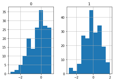
we might notice that variable X0 has a cliff at 1. We may correctly suspect that all values above 1 were cencored.
How might we distinguish between the X_MAR and the X_MCAR
datasets if we did not already know how they were simulated? In Pandas,
we can test which entries are missing with isna, notna.
X_MCAR.isna().head()
| 0 | 1 | |
|---|---|---|
| 0 | False | False |
| 1 | False | False |
| 2 | True | False |
| 3 | False | False |
| 4 | False | False |
This converted all of the entries to the True/False answer to “is this
value missing?”. This is the preferred way to evaluate missingness
because in Python np.nan == np.nan actually evaluates to False, so
testing with expressions of this type doesn’t work.
You should think of the result of isna as another variable that you
may want to include in your analysis. In prediction tasks we will often
include these variables when we do feature engineering, as we will see
later. For our purposes, we can see the difference between the X_MAR
and X_MCAR data with this missingness indicator included.
Specifically, we want to see what the dependence is between the
missingness and other variables. We can do this by grouping by the
missingness and describing the other variable. The following function
adds the missingness indicator to a dataset for a variable, removes that
variable, groups by the missingness, and describes the remaining
variables.
def desc_missing(X,missingvar):
    """Describes the variables conditioned on the missingness"""
    X_mod = X.copy()
    X_mod['miss_ind'] = X_mod[missingvar].isna()
    del X_mod[missingvar]
    return X_mod.groupby('miss_ind').describe()
desc_missing(X_MCAR,0)
| 1 | ||||||||
|---|---|---|---|---|---|---|---|---|
| count | mean | std | min | 25% | 50% | 75% | max | |
| miss_ind | ||||||||
| False | 170.0 | -0.059364 | 0.939388 | -2.403688 | -0.577253 | -0.046619 | 0.575143 | 2.643257 |
| True | 30.0 | -0.034340 | 1.023837 | -2.152632 | -0.632773 | 0.029868 | 0.724111 | 1.795847 |
desc_missing(X_MAR,0)
| 1 | ||||||||
|---|---|---|---|---|---|---|---|---|
| count | mean | std | min | 25% | 50% | 75% | max | |
| miss_ind | ||||||||
| False | 172.0 | -0.255640 | 0.790491 | -2.568347 | -0.695704 | -0.102948 | 0.379905 | 0.982192 |
| True | 28.0 | 1.480858 | 0.416369 | 1.069409 | 1.218558 | 1.365086 | 1.586109 | 3.018901 |
In the above displays, we see that for the MCAR dataset there is little
difference between the summary statistics for X1 when X0 is missing or
not. For the MAR dataset, there is a more pronounced difference between
the means of these two subsets of the data. This is one indication to us
that X_MAR is not MCAR.
We could also do this formally with a T-test for difference in means between two samples to do this more formally. I will assume that you recall the T-test for independence from your introductory statistics course, if not please review it before trying to parse the following code blocks.
def test_MCAR(X,missingvar,testvar):
    """
    Test if testvar is independent of missingness
    Uses two-sided t-test with pooled variances
    """
    X_mod = X.copy()
    X_mod['miss_ind'] = X_mod[missingvar].isna()
    del X_mod[missingvar]
    X1,X2 = [df for i,df in X_mod.groupby('miss_ind')] #split
    return sm.stats.ttest_ind(X1[testvar],X2[testvar]) #return test
In the above function we split the grouped dataframe based on the
missingness status. We used the ttest_ind method in statsmodels to
perform the two-sample t-test with pooled variances. The resulting
P-values are below:
print("X_MCAR P-value: {}".format(test_MCAR(X_MCAR,0,1)[1]))
print("X_MAR P-value: {}".format(test_MCAR(X_MAR,0,1)[1]))
X_MCAR P-value: 0.8945613701172417
X_MAR P-value: 2.4792949402817898e-23
This provides more satisfying evidence that the dataset X_MAR is not
drawn MCAR.
Dealing with missingness and simple imputation
Imputation is the process of filling in missing values. There are few great options when it comes to imputation, and very few general purpose tools that will perfectly impute missing data. Let’s discuss some reasonable simple options and their limitations.
Let’s begin by loading in the Melbourne housing dataset, which is from the Kaggle competitions: https://www.kaggle.com/anthonypino/melbourne-housing-market/version/26 The dataset describes home sales in Melborne, Australia.
mel = pd.read_csv('../data/Melbourne_housing_FULL.csv')
mel.head()
| Suburb | Address | Rooms | Type | Price | Method | SellerG | Date | Distance | Postcode | ... | Bathroom | Car | Landsize | BuildingArea | YearBuilt | CouncilArea | Lattitude | Longtitude | Regionname | Propertycount | |
|---|---|---|---|---|---|---|---|---|---|---|---|---|---|---|---|---|---|---|---|---|---|
| 0 | Abbotsford | 68 Studley St | 2 | h | NaN | SS | Jellis | 3/09/2016 | 2.5 | 3067.0 | ... | 1.0 | 1.0 | 126.0 | NaN | NaN | Yarra City Council | -37.8014 | 144.9958 | Northern Metropolitan | 4019.0 |
| 1 | Abbotsford | 85 Turner St | 2 | h | 1480000.0 | S | Biggin | 3/12/2016 | 2.5 | 3067.0 | ... | 1.0 | 1.0 | 202.0 | NaN | NaN | Yarra City Council | -37.7996 | 144.9984 | Northern Metropolitan | 4019.0 |
| 2 | Abbotsford | 25 Bloomburg St | 2 | h | 1035000.0 | S | Biggin | 4/02/2016 | 2.5 | 3067.0 | ... | 1.0 | 0.0 | 156.0 | 79.0 | 1900.0 | Yarra City Council | -37.8079 | 144.9934 | Northern Metropolitan | 4019.0 |
| 3 | Abbotsford | 18/659 Victoria St | 3 | u | NaN | VB | Rounds | 4/02/2016 | 2.5 | 3067.0 | ... | 2.0 | 1.0 | 0.0 | NaN | NaN | Yarra City Council | -37.8114 | 145.0116 | Northern Metropolitan | 4019.0 |
| 4 | Abbotsford | 5 Charles St | 3 | h | 1465000.0 | SP | Biggin | 4/03/2017 | 2.5 | 3067.0 | ... | 2.0 | 0.0 | 134.0 | 150.0 | 1900.0 | Yarra City Council | -37.8093 | 144.9944 | Northern Metropolitan | 4019.0 |
5 rows × 21 columns
mel.info()
<class 'pandas.core.frame.DataFrame'>
RangeIndex: 34857 entries, 0 to 34856
Data columns (total 21 columns):
Suburb           34857 non-null object
Address          34857 non-null object
Rooms            34857 non-null int64
Type             34857 non-null object
Price            27247 non-null float64
Method           34857 non-null object
SellerG          34857 non-null object
Date             34857 non-null object
Distance         34856 non-null float64
Postcode         34856 non-null float64
Bedroom2         26640 non-null float64
Bathroom         26631 non-null float64
Car              26129 non-null float64
Landsize         23047 non-null float64
BuildingArea     13742 non-null float64
YearBuilt        15551 non-null float64
CouncilArea      34854 non-null object
Lattitude        26881 non-null float64
Longtitude       26881 non-null float64
Regionname       34854 non-null object
Propertycount    34854 non-null float64
dtypes: float64(12), int64(1), object(8)
memory usage: 5.6+ MB
From the count we can see that there is significant missingness in many of these variables. While we would like to impute as many of these values as possible, we are especially interested in imputing the Price of the home. Before we proceed with this, we can notice that Date and YearBuilt columns are not datetimes, so we should convert these first.
mel['Date'][:5]
0    3/09/2016
1    3/12/2016
2    4/02/2016
3    4/02/2016
4    4/03/2017
Name: Date, dtype: object
Looking at the Date, we can see that the string is in a standard date format, and we can then cast as a datetime.
mel['Date'] = pd.to_datetime(mel['Date'],format="%d/%m/%Y")
The Yearbuilt variable is a bit more challenging, since it was cast as a float.
mel['YearBuilt'][:5]
0       NaN
1       NaN
2    1900.0
3       NaN
4    1900.0
Name: YearBuilt, dtype: float64
Let’s write a custom function that converts the float first to integer, then to string, if it is not NaN.
def conv_year(y):
    if np.isnan(y):
        return np.nan
    return str(int(y))
We apply this using the apply method, then convert to a PeriodIndex
object.
mel['YearBuilt'] = mel['YearBuilt'].apply(conv_year)
mel['YearBuilt'] = pd.PeriodIndex(mel['YearBuilt'],freq="Y")
We can verify that this is the desired result.
mel['YearBuilt'][:5]
0    NaT
1    NaT
2   1900
3    NaT
4   1900
Name: YearBuilt, dtype: object
We have seen the use of isna to make a missingness indicator
variable. We can easily do this to all of the variables and add
missingness indicators for all of them using a join.
mel_miss = mel.isna()
mel = mel.join(mel_miss,rsuffix="_miss")
Now mel has twice the number of columns.
mel.columns
Index(['Suburb', 'Address', 'Rooms', 'Type', 'Price', 'Method', 'SellerG',
       'Date', 'Distance', 'Postcode', 'Bedroom2', 'Bathroom', 'Car',
       'Landsize', 'BuildingArea', 'YearBuilt', 'CouncilArea', 'Lattitude',
       'Longtitude', 'Regionname', 'Propertycount', 'Suburb_miss',
       'Address_miss', 'Rooms_miss', 'Type_miss', 'Price_miss', 'Method_miss',
       'SellerG_miss', 'Date_miss', 'Distance_miss', 'Postcode_miss',
       'Bedroom2_miss', 'Bathroom_miss', 'Car_miss', 'Landsize_miss',
       'BuildingArea_miss', 'YearBuilt_miss', 'CouncilArea_miss',
       'Lattitude_miss', 'Longtitude_miss', 'Regionname_miss',
       'Propertycount_miss'],
      dtype='object')
The simplest form of imputation is to replace the missing values in a
column with a single value. This can be accomplished with fillna
which can take either a single value or a Series. The Series in this
case has to have keys which are the column names to be filled, and the
values are what to fill with.
For example, suppose that for all of the float columns we want to impute
with the median, and for all of the rest we want to impute with the
mode. We can use the select_dtypes to select the columns of a
certain type.
imp_values = mel.select_dtypes(exclude=float).mode().loc[0] # mode returns a DataFrame
imp_values = imp_values.append(mel.select_dtypes(include=float).median())
We used append to combine the two resulting Series to give us the
following,
imp_values
Suburb                              Reservoir
Address                          5 Charles St
Rooms                                       3
Type                                        h
Method                                      S
SellerG                                Jellis
Date                      2017-10-28 00:00:00
YearBuilt                                1970
CouncilArea           Boroondara City Council
Regionname              Southern Metropolitan
Suburb_miss                             False
Address_miss                            False
Rooms_miss                              False
Type_miss                               False
Price_miss                              False
Method_miss                             False
SellerG_miss                            False
Date_miss                               False
Distance_miss                           False
Postcode_miss                           False
Bedroom2_miss                           False
Bathroom_miss                           False
Car_miss                                False
Landsize_miss                           False
BuildingArea_miss                        True
YearBuilt_miss                           True
CouncilArea_miss                        False
Lattitude_miss                          False
Longtitude_miss                         False
Regionname_miss                         False
Propertycount_miss                      False
Price                                  870000
Distance                                 10.3
Postcode                                 3103
Bedroom2                                    3
Bathroom                                    2
Car                                         2
Landsize                                  521
BuildingArea                              136
Lattitude                            -37.8076
Longtitude                            145.008
Propertycount                            6763
dtype: object
Now we are prepared to impute with these values. We are only going to impute with this simple scheme when CouncilArea is missing however, which we will explain shortly.
ca_na = mel['CouncilArea'].isna()
mel[ca_na] = mel[ca_na].fillna(imp_values)
We will impute using the CouncilArea as a predictor, but when it is missing we will need to impute using a single value for each column. There are only three rows with missing CouncilArea though, so this is just for completeness sake. For comparison purposes however, we can make a copy of the Price and look at the distribution before and after imputation with a single value.
price = mel['Price'].copy()
We will first look at the histogram of Price when it is non-missing. We can see from the imputed value above that the median is 870,000 AUD.
price.hist(bins=40)
plt.title('Histogram of Price: non-missing')
plt.show()
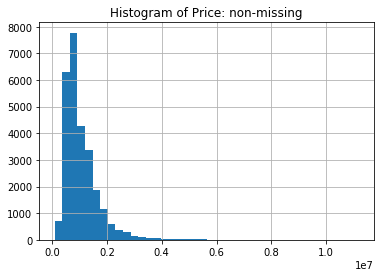
Contrasting this with the histogram of the Price after we impute with the median for the non-missing, we see one immediate deficiency of imputing with a single value.
price.fillna(imp_values['Price']).hist(bins=40)
plt.title('Histogram of Price: single value imputation')
plt.show()
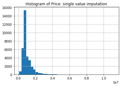
The histogram now has a spike at the imputed value. This indicates that if we impute with a single value then the sample distribution will have a point mass. Imputing with the median will preserve the median, but statistics regarding the spread of the distribution will be lower, for example, compare the median and standard deviation below (50% and std).
price.describe()
count    2.724700e+04
mean     1.050173e+06
std      6.414671e+05
min      8.500000e+04
25%      6.350000e+05
50%      8.700000e+05
75%      1.295000e+06
max      1.120000e+07
Name: Price, dtype: float64
price.fillna(imp_values['Price']).describe()
count    3.485700e+04
mean     1.010838e+06
std      5.719992e+05
min      8.500000e+04
25%      6.950000e+05
50%      8.700000e+05
75%      1.150000e+06
max      1.120000e+07
Name: Price, dtype: float64
If we would like to get a more plausible sample distribution for the Price after imputation, then we have two choices: multiple imputation (which we will not go into) and imputation using prediction.
In Pandas, you can also use fillna to impute with a time series by
filling in the entries by padding from a given value. This type of
padding can be done in a forward or backward fashion. While we could use
Date to impute the Price, it will likely be more effective to use either
locational information or all of the continuous/ordinal variables
including Date.
Imputation by Prediction
Recall that if a variable is MCAR then looking at the other variables should not help the imputation process. If the Price is MAR then we can impute by thinking of this as a prediction problem, with all other variables and their missingness statuses as predictors and the Price as a response.
We will first impute all of the variables using CouncilArea as the sole predictor. We can simply think of this as grouping by the CouncilArea and then imputing with a single value for that group and column. CouncilArea is a good choice as a variable to condition on since it is mostly non-missing, and as we will see in the next code block, when we group by the CouncilArea there are no columns that are all missing in a group. Hence, if we want to impute with the median or mode within a group, this will always be well defined.
ca_groupct = mel.groupby('CouncilArea').count()
(ca_groupct == 0).any().any()
# is there any column that is all NaN for any council?
False
In order to impute within groups we will combine the groupby method
with the transform. The idea is that we want to make a
transformation within each group, and this can be accomplished in the
following way. But we first need to create a function that defines how
we want to impute within the groups (which is the tranformation that
needs to be applied).
def impute_med(x):
    """impute NaNs for Series x with median if it is a float and mode otherwise"""
    if x.dtype == float:
        return x.fillna(x.median())
    if x.name  == "YearBuilt":
        return x.fillna(x.mode()[0])
    return x.fillna(x.mode())
In the above transformation, we test if the Series has a float dtype,
and if so fill the NaNs with the median, otherwise we use the mode. The
YearBuild variable is causing some troubles because the mode returns a
Series and not a single value, so we will deal with that variable
specifically by looking at the name of the Series.
CA = mel['CouncilArea'].copy() # the process does not preserve CouncilArea, save it
mel[~ca_na] = mel[~ca_na].groupby('CouncilArea').transform(impute_med)
mel['CouncilArea'] = CA # rewrite CouncilArea
We can see that now all values have been imputed.
mel.info()
<class 'pandas.core.frame.DataFrame'>
RangeIndex: 34857 entries, 0 to 34856
Data columns (total 42 columns):
Suburb                34857 non-null object
Address               34857 non-null object
Rooms                 34857 non-null int64
Type                  34857 non-null object
Price                 34857 non-null float64
Method                34857 non-null object
SellerG               34857 non-null object
Date                  34857 non-null datetime64[ns]
Distance              34857 non-null float64
Postcode              34857 non-null float64
Bedroom2              34857 non-null float64
Bathroom              34857 non-null float64
Car                   34857 non-null float64
Landsize              34857 non-null float64
BuildingArea          34857 non-null float64
YearBuilt             34857 non-null object
CouncilArea           34857 non-null object
Lattitude             34857 non-null float64
Longtitude            34857 non-null float64
Regionname            34857 non-null object
Propertycount         34857 non-null float64
Suburb_miss           34857 non-null bool
Address_miss          34857 non-null bool
Rooms_miss            34857 non-null bool
Type_miss             34857 non-null bool
Price_miss            34857 non-null bool
Method_miss           34857 non-null bool
SellerG_miss          34857 non-null bool
Date_miss             34857 non-null bool
Distance_miss         34857 non-null bool
Postcode_miss         34857 non-null bool
Bedroom2_miss         34857 non-null bool
Bathroom_miss         34857 non-null bool
Car_miss              34857 non-null bool
Landsize_miss         34857 non-null bool
BuildingArea_miss     34857 non-null bool
YearBuilt_miss        34857 non-null bool
CouncilArea_miss      34857 non-null bool
Lattitude_miss        34857 non-null bool
Longtitude_miss       34857 non-null bool
Regionname_miss       34857 non-null bool
Propertycount_miss    34857 non-null bool
dtypes: bool(21), datetime64[ns](1), float64(11), int64(1), object(8)
memory usage: 6.3+ MB
Again, we can look at the histogram,
mel['Price'].hist(bins=40)
plt.title("Histogram of Price: imputed by CouncilArea")
plt.show()
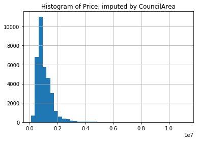
While there seems to be a larger spike around 1M AUD, the sample distribution does look more like the original sample distribution.
We have seen how you can impute with a categorical variable as the
predictor using groupby. We can also think about using the other
variables, particularly the numerical variables, in a linear regressor.
Before we do this however, we would like to compare prediction with the
numerical variables against predicting with CouncilArea. To do this
let’s make a training and testing split of the observed Price data
(using the Price_miss variable). We will see the sklearn package
later, but for now, we will just import the train_test_split
function. This makes a randomized split of the data with a default of a
3:1 ratio for train and test sets respectively.
from sklearn.model_selection import train_test_split

train, test = train_test_split(mel[~mel['Price_miss']])
We will extract the predictions in the form of a Series with the CouncilArea as the index and the mean Price within that CouncilArea as the values.
ca_na = train['CouncilArea_miss']
tr_preds = train[~ca_na][['CouncilArea','Price']].groupby('CouncilArea').mean()
We will then join this series to the full Price data with the CouncilArea as the index. Notice that the left DataFrame is much larger and has many duplicate indices, while the indices in the right DataFrame are unique. Because this is a left join, the right Dataframe rows will be multiplied to match the multiple rows on the left.
test_dat = test[['CouncilArea','Price']]
test_dat = test_dat.set_index('CouncilArea')
test_dat = test_dat.join(tr_preds,rsuffix='_pred')
We can look at the result and see that the behavior is as expected, the
Price_pred is dependent on the CouncilArea.
test_dat.head()
| Price | Price_pred | |
|---|---|---|
| CouncilArea | ||
| Banyule City Council | 1278000.0 | 942259.175601 |
| Banyule City Council | 845000.0 | 942259.175601 |
| Banyule City Council | 985000.0 | 942259.175601 |
| Banyule City Council | 690000.0 | 942259.175601 |
| Banyule City Council | 728500.0 | 942259.175601 |
We can simply calculate the square error test error using the eval
method. We have not gone over the eval method, but it is often
handy. Since the columns are named, we can write mathematical
expressions using them, then eval will evaluate it for every row of
the DataFrame. We then calculate the mean.
CA_error = test_dat.eval('(Price - Price_pred)**2').mean()
CA_error
312621748714.5273
Let’s consider using linear regression to predict the Price instead. We will create a handy function to select the desired predictor and response DataFrames below. We will exclude the non-numeric variables from the predictors. Critically, the missingness indicators are all included as predictor variables. We also cast the result as Numpy Arrrays with dtype of float.
def select_preds(train):
    """"""
    X_tr = train.select_dtypes(include=[float,bool,int])
    Y_tr = X_tr['Price'].copy()
    del X_tr['Price']
    names = list(X_tr.columns)
    X_tr, Y_tr = X_tr.astype(float), Y_tr.astype(float)
    return Y_tr, X_tr
We then apply this to the train and test sets and fit OLS and predict on the test set.
Y_tr, X_tr = select_preds(train)
Y_te, X_te = select_preds(test)
ols_res = sm.OLS(Y_tr,X_tr).fit()
Y_pred = ols_res.predict(X_te)
ols_res.summary()
| Dep. Variable: | Price | R-squared: | 0.852 |
|---|---|---|---|
| Model: | OLS | Adj. R-squared: | 0.852 |
| Method: | Least Squares | F-statistic: | 5871. |
| Date: | Thu, 20 Sep 2018 | Prob (F-statistic): | 0.00 |
| Time: | 09:42:51 | Log-Likelihood: | -2.9610e+05 |
| No. Observations: | 20435 | AIC: | 5.922e+05 |
| Df Residuals: | 20415 | BIC: | 5.924e+05 |
| Df Model: | 20 | ||
| Covariance Type: | nonrobust |
| coef | std err | t | P>|t| | [0.025 | 0.975] | |
|---|---|---|---|---|---|---|
| Rooms | 3.419e+05 | 6794.377 | 50.315 | 0.000 | 3.29e+05 | 3.55e+05 |
| Distance | -4.733e+04 | 604.181 | -78.341 | 0.000 | -4.85e+04 | -4.61e+04 |
| Postcode | 1160.6889 | 35.744 | 32.472 | 0.000 | 1090.628 | 1230.750 |
| Bedroom2 | -3.49e+04 | 8042.990 | -4.339 | 0.000 | -5.07e+04 | -1.91e+04 |
| Bathroom | 1.741e+05 | 6443.674 | 27.020 | 0.000 | 1.61e+05 | 1.87e+05 |
| Car | 5.412e+04 | 4224.249 | 12.812 | 0.000 | 4.58e+04 | 6.24e+04 |
| Landsize | 4.1204 | 0.998 | 4.128 | 0.000 | 2.164 | 6.077 |
| BuildingArea | 60.9449 | 10.398 | 5.861 | 0.000 | 40.565 | 81.325 |
| Lattitude | -1.258e+06 | 4.03e+04 | -31.204 | 0.000 | -1.34e+06 | -1.18e+06 |
| Longtitude | -3.509e+05 | 1.05e+04 | -33.521 | 0.000 | -3.71e+05 | -3.3e+05 |
| Propertycount | -1.3879 | 0.743 | -1.868 | 0.062 | -2.844 | 0.069 |
| Suburb_miss | 6.778e-08 | 2.01e-08 | 3.380 | 0.001 | 2.85e-08 | 1.07e-07 |
| Address_miss | -2.664e-07 | 7.85e-08 | -3.395 | 0.001 | -4.2e-07 | -1.13e-07 |
| Rooms_miss | 4.365e-07 | 1.29e-07 | 3.395 | 0.001 | 1.84e-07 | 6.88e-07 |
| Type_miss | 5.8e-08 | 1.71e-08 | 3.395 | 0.001 | 2.45e-08 | 9.15e-08 |
| Price_miss | 1.287e-08 | 3.8e-09 | 3.390 | 0.001 | 5.43e-09 | 2.03e-08 |
| Method_miss | -2.877e-08 | 8.5e-09 | -3.385 | 0.001 | -4.54e-08 | -1.21e-08 |
| SellerG_miss | -2.241e-08 | 6.49e-09 | -3.452 | 0.001 | -3.51e-08 | -9.68e-09 |
| Date_miss | -1.267e-08 | 3.77e-09 | -3.365 | 0.001 | -2.01e-08 | -5.29e-09 |
| Distance_miss | -1.75e+05 | 2.91e+05 | -0.601 | 0.548 | -7.45e+05 | 3.95e+05 |
| Postcode_miss | -1.75e+05 | 2.91e+05 | -0.601 | 0.548 | -7.45e+05 | 3.95e+05 |
| Bedroom2_miss | -1.244e+06 | 3.38e+05 | -3.677 | 0.000 | -1.91e+06 | -5.81e+05 |
| Bathroom_miss | 1.109e+06 | 3.37e+05 | 3.289 | 0.001 | 4.48e+05 | 1.77e+06 |
| Car_miss | 7.084e+04 | 2.85e+04 | 2.484 | 0.013 | 1.5e+04 | 1.27e+05 |
| Landsize_miss | -1.822e+04 | 1.12e+04 | -1.630 | 0.103 | -4.01e+04 | 3691.804 |
| BuildingArea_miss | 1.264e+04 | 1.25e+04 | 1.015 | 0.310 | -1.18e+04 | 3.71e+04 |
| YearBuilt_miss | 4.737e+04 | 1.26e+04 | 3.757 | 0.000 | 2.27e+04 | 7.21e+04 |
| CouncilArea_miss | -4.717e+04 | 1.12e+05 | -0.421 | 0.674 | -2.67e+05 | 1.72e+05 |
| Lattitude_miss | -1.956e+04 | 1.89e+04 | -1.034 | 0.301 | -5.66e+04 | 1.75e+04 |
| Longtitude_miss | -1.956e+04 | 1.89e+04 | -1.034 | 0.301 | -5.66e+04 | 1.75e+04 |
| Regionname_miss | -4.717e+04 | 1.12e+05 | -0.421 | 0.674 | -2.67e+05 | 1.72e+05 |
| Propertycount_miss | -4.717e+04 | 1.12e+05 | -0.421 | 0.674 | -2.67e+05 | 1.72e+05 |
| Omnibus: | 13579.846 | Durbin-Watson: | 2.004 |
|---|---|---|---|
| Prob(Omnibus): | 0.000 | Jarque-Bera (JB): | 485785.597 |
| Skew: | 2.698 | Prob(JB): | 0.00 |
| Kurtosis: | 26.269 | Cond. No. | 1.20e+16 |
Warnings:
[1] Standard Errors assume that the covariance matrix of the errors is correctly specified.
[2] The smallest eigenvalue is 1.21e-20. This might indicate that there are
strong multicollinearity problems or that the design matrix is singular.
There seem to be many strong predictors in the OLS, particularly, variables like Rooms, Distance, Cars, Bathroom, but also the missingness indicators seem to have some predictive power. Interestingly the postal code is also predictive in a linear model, even though using the postal code as a numerical variable in linear regression does not make much sense, although nearby postal codes do tend to be close geographically.
Regardless, because we are doing a train-test split, we can feel confident that the resulting test error is a good estimate of the risk of the prediction.
ols_error = np.mean((Y_pred - Y_te)**2)
ols_error / CA_error
0.7162549957690686
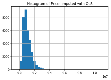
We see that the test error from the OLS is 71.6% of the prediction from the CouncilArea, and we can confidently use the OLS prediction to impute the missing Prices.
Y, X = select_preds(mel[~mel['Price_miss']])
_, X_miss = select_preds(mel[mel['Price_miss']])
ols_res = sm.OLS(Y,X).fit()
Y_pred = ols_res.predict(X_miss)
mel.loc[mel['Price_miss'],'Price'] = Y_pred
We have used more basic Pandas indexing and assignment to do the imputation above. Try to follow the precise operations we have performed. As usual, we can look at the sample distribution for the resulting imputation.
mel['Price'].hist(bins=40)
plt.title("Histogram of Price: imputed with OLS")
plt.show()